Cancer Networks and Variant Data

This protocol will demonstrate network retrieval from the STRING database, basic analysis, TCGA data loading and visualization in Cytoscape.

Setup

• Install the stringApp and Diffusion apps from the Cytoscape App Store, or install from Cytoscape via Apps → App Store → Open App Store

Getting Disease Networks

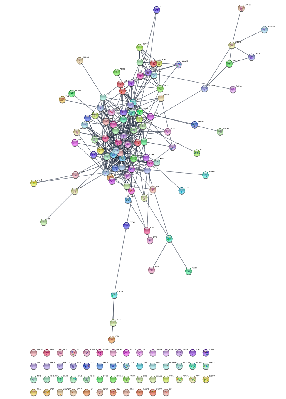
We are going to query the STRING database from Cytoscape to retrieve networks of genes associated with breast cancer.

• In the Network Search bar at the top of the Network Panel, select STRING disease query from the drop-down, and type in breast cancer.
• Click the options icon and set the Confidence (score) cutoff to 0.9 and the Maximum number of proteins to 150.
• Click the search icon to search.

Learn more about using STRING

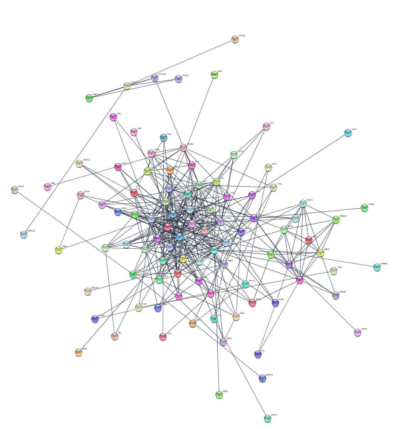
Layout Network

We can apply a layout algorithm to help visualize the network. Cytoscape supports a large collection of automatic layout algorithms, available under the Layout menu. For this layout, we are going to change the default parameters a bit first:

• Open the Layout Settings by selecting Layout → Settings....
• Under Layout Algorithm, select Prefuse Force Directed.
• Set the Default Spring Coefficient to 8E-7 and the Default Spring Length to 70.
• Click Apply Layout.

The largest component of the network will look like this:

Learn more about Layouts

Generate Subnetworks

To explore the network, we can use various parameters of the network to generate relevant subnetworks. Let's start by creating a network from a subset of nodes with a high disease score:

• Click on the Filter tab of the Control Panel.
• Click on the drop-down to the right and select Create New Filter.
• Click the + (add) button and select Column Filter. In the Choose column... drop-down, select Node: disease score.
• In the selection slider, select scores of 3.3 or higher. This will select around 40 nodes.
• With the nodes still selected, go to File → New Network → From Selected Nodes, All Edges.

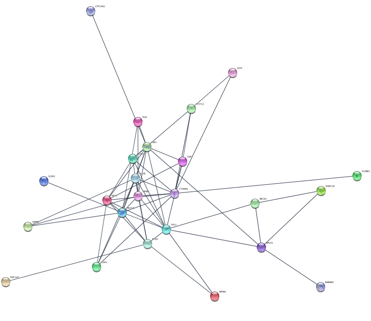
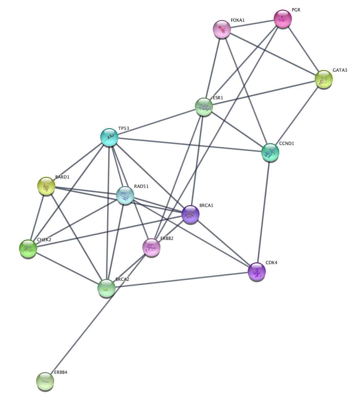
This will create a subnetwork with a connected component and some unconnected nodes. We can delete the extra nodes by selecting them with click-and-drag and clicking Delete.

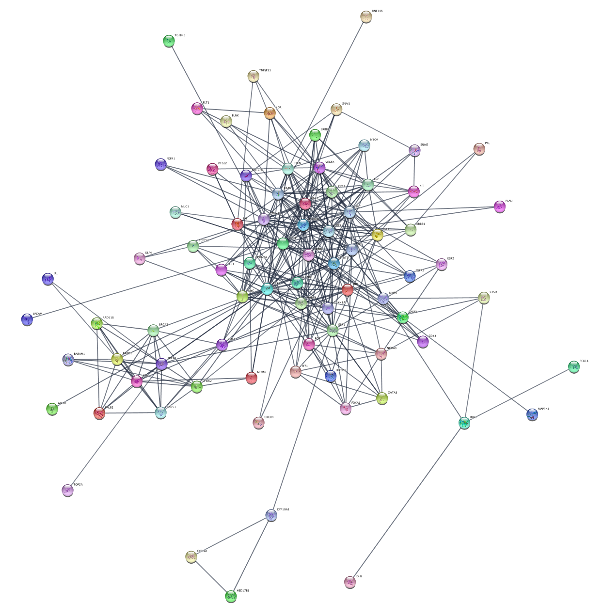
Generate Subnetworks

Another strategy is to create a subnetwork from first neighbors of genes with the highest disease score, using the network connectivity together with the data to direct discovery.

• In the original String breast cancer network, reapply the disease score > 3.3 filter, unless the relevant nodes are still selected.
• With the nodes selected, go to Select → Nodes → Select First Neighbors of Selected Nodes → Undirected.
• With the nodes still selected, go to File → New Network → From Selected Nodes, All Edges.

Generate Subnetworks

The Diffusion app uses the network connectivity in a more subtle way than just first-degree neighbors. We can combine this with the top scoring genes:

• Again, select the original String breast cancer network. Click anywhere on the canvas to undo the current node selection.
• In the Filter tab, adjust the threshold for the disease score column filter to select nodes with a score of 4.2 and above. This will select a small number of top nodes.
• With the nodes selected, select Tools → Diffuse → Selected Nodes.
• The Diffusion results will open in the Results Panel. Click Create to create a subnetwork.
• Apply the Prefuse Force Directed layout.

Learn more about Filtering by Selection

Visualizing Data

From the TCGA, we have access to mutation data and expression data for breast cancer. We can visualize this data on the network, and also use it for analysis.

• Select the second subnetwork, representing nodes with disease score of 3.3 or higher and their first neighbors.
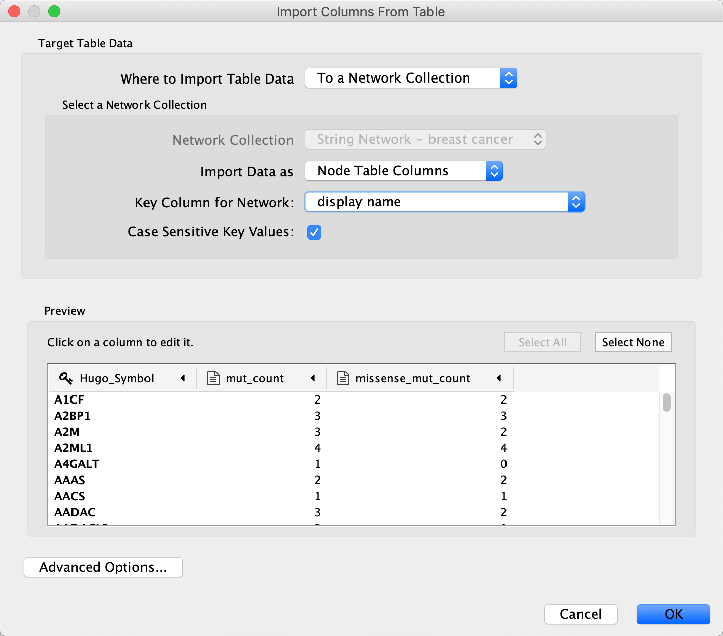
• Load the mutation data file file under File menu, select Import → Table from File.....
• For this data, the Key Column for Network should be set to display name to match the Hugo symbol used in the data.
• Repeat the import process for the expression data file, again mapping through the display name.

Visualizing Data

Let’s create a new style to visualize our imported data.

• In the Style tab in the Control Panel, click the Options icon and select Create New Style.... Name your new style data style.
• Change the default node shape to ellipse and check Lock node width and height.
• Set the default node Size to 60.
• Set the default node Fill Color to gray.
• Set the default edge Width to 2.
• Create a Passthrough Mapping for node Label to display name.

Visualizing Data

Now we can add a mapping for mean expression.

• Create a Continuous Mapping for node Fill Color to expr.mean, using the default blue-red gradient.

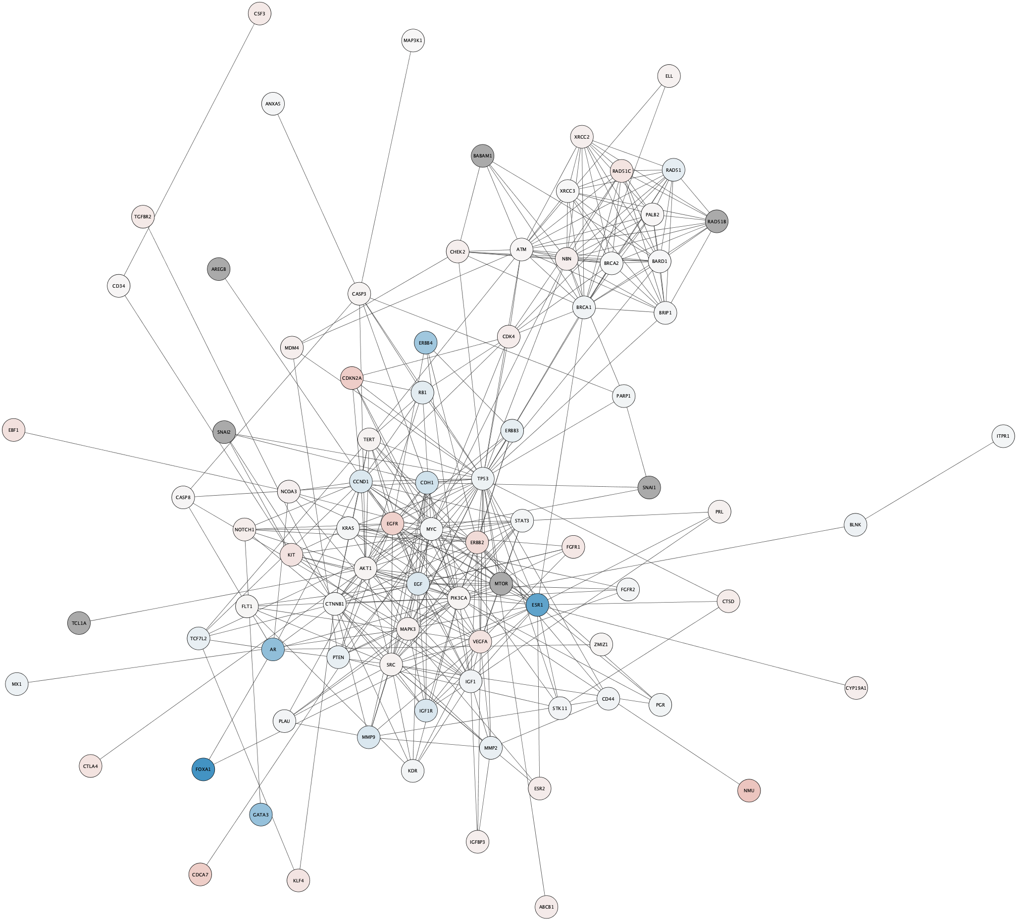
Visualizing Data

Finally, we can add a mapping for mutation data.

• Create a Continuous Mapping for node Border Width to mut_count, with node border width from 2 to 8.
• Create a Continuous Mapping for node Border Paint to mut_count, using the ColorBrewer Red palette.

This is a useful pair of visual properties to map to a single data column. See why?

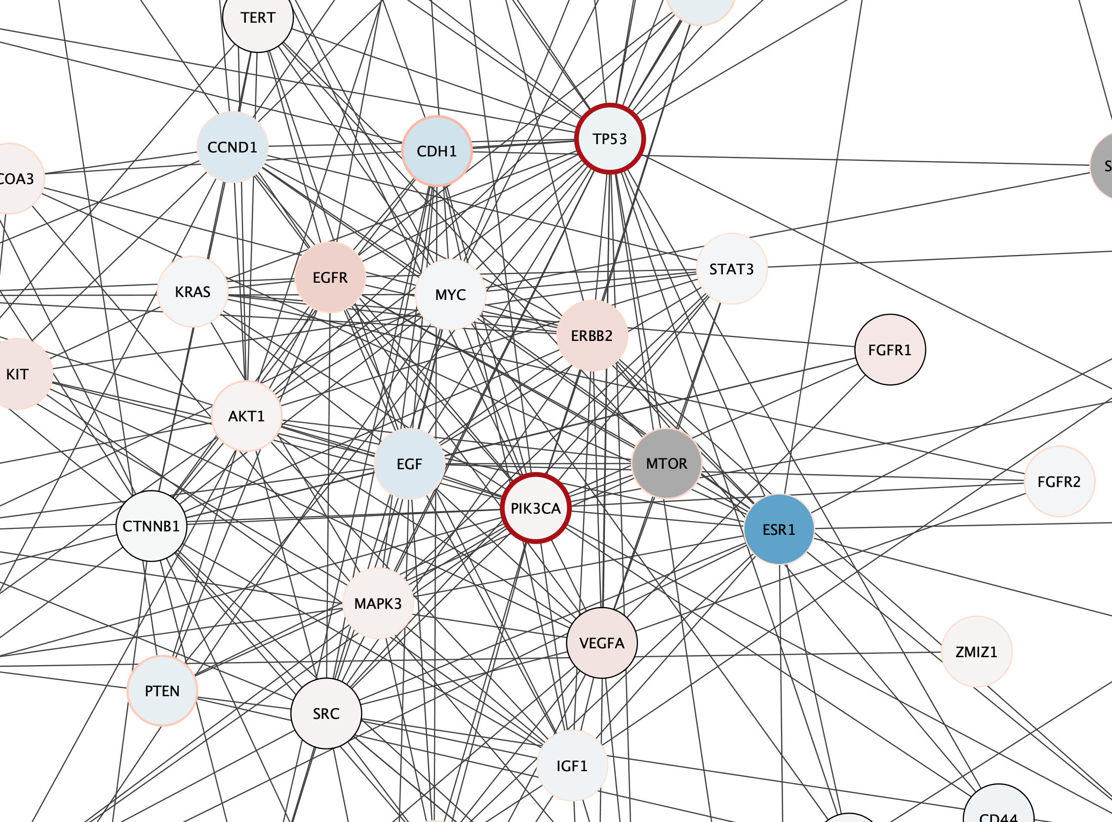
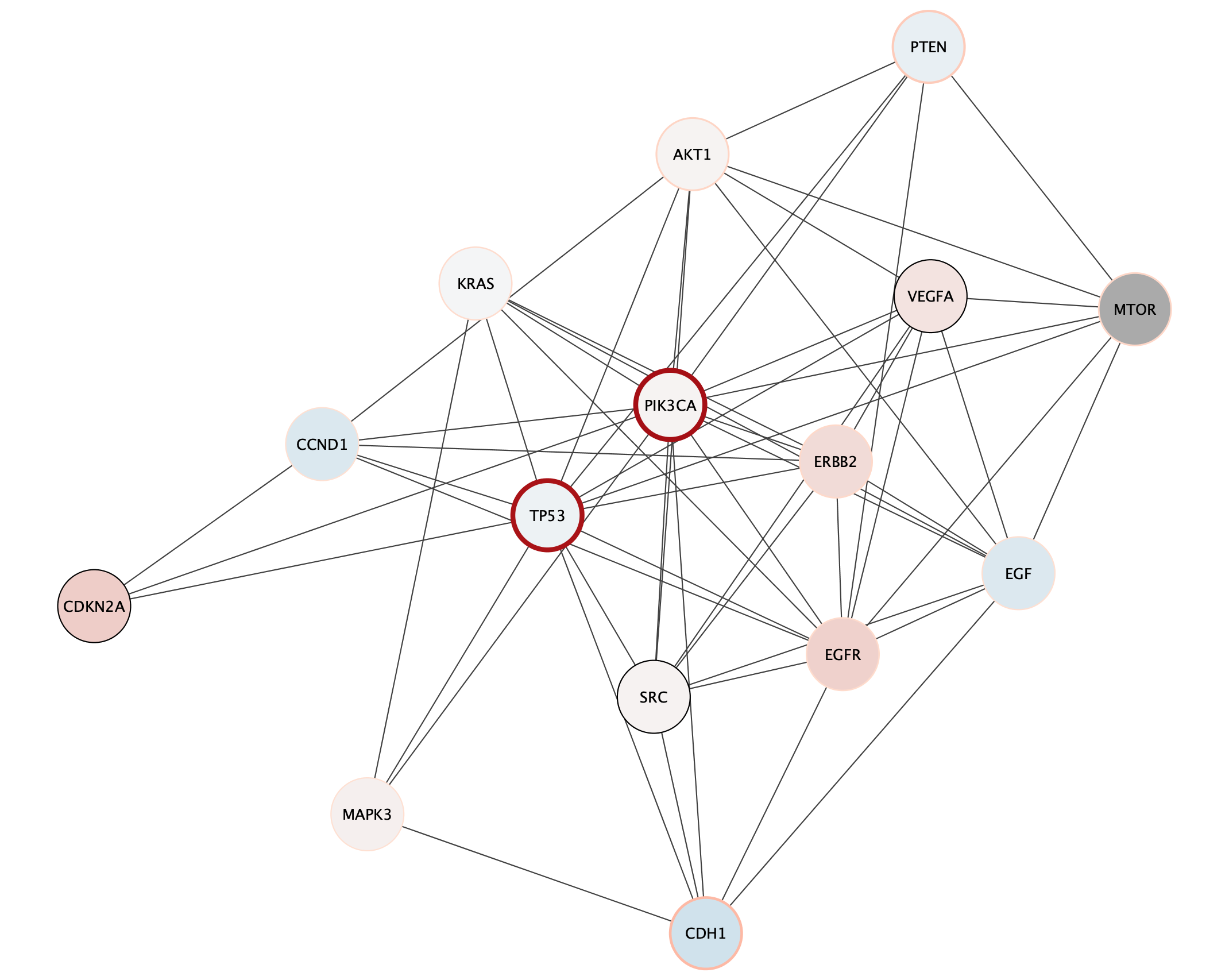
Subnetwork Based on Diffusion from Heavily Mutated Nodes

We can now combine our earlier strategy for subnetwork selection with the mutation data, by using the Diffusion algorithm on the top mutated genes.

• The top two mutated genes in this network are TP53 and PIK3CA. Select these two nodes.
• With the nodes selected, select Tools → Diffuse → Selected Nodes.
• The Diffusion results will open in the Results Panel. Click Create to create a subnetwork.
• The subnetwork may open with the default visual style. In the Style tab, select the data style that we created earlier.
• Apply the Prefuse Force Directed layout.

Subnetwork Based on Diffusion from Heavily Mutated Nodes

The top mutated genes are based on TCGA data and the diffusion algorithm is operating based on the network connectivity from STRING data, leading to a focused subnetwork view of critical breast cancer genes with mean patient expression data mapped to fill color. Now that’s data integration!

Exporting Networks

Cytoscape provides a number of ways to save results and visualizations:

• As a session: File → Save Session, File → Save Session As...
• As an image: File → Export → Network to Image...
• To the web: File → Export → Network to Web Page... (Example)
• To a public repository: File → Export → Network to NDEx
• As a graph format file: File → Export → Network to File.
  Formats:
  • CX JSON / CX2 JSON
  • Cytoscape.js JSON
  • GraphML
  • PSI-MI
  • XGMML
  • SIF